KNN - You’ve heard about it, but what is it?
K-NearestNeighbors, often called KNN for short, is a machine learning model used to generate predictions. And those predictions can be scored, outputting a percentage of how well the model did.
I’ll be using the Breast Cancer Wisconsin (Original) Data Set from UCI, but first lets go over some basics.
Starting Small
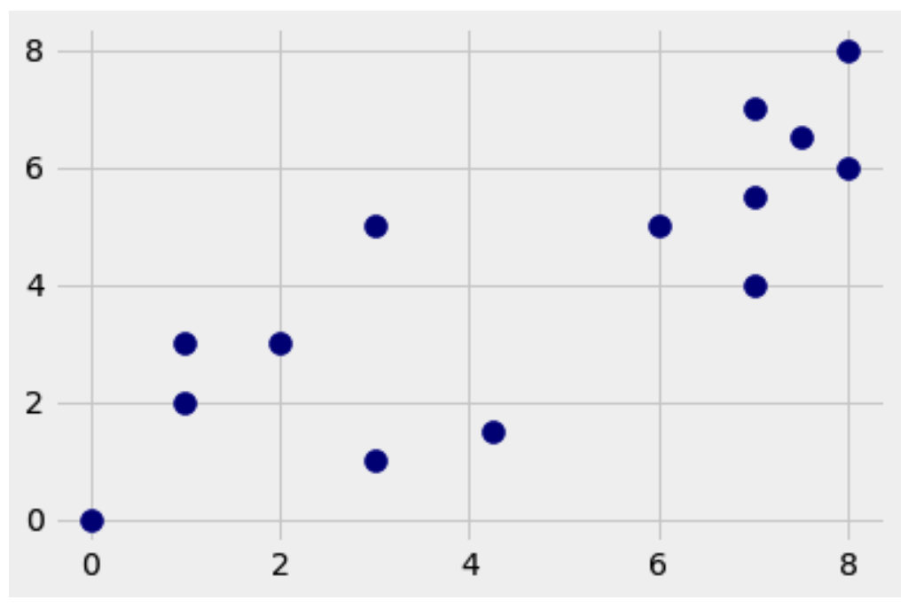
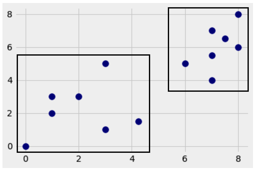
Here is a small, fake dataset with 14 dots. Are you able to make two groups out of them?
import matplotlib.pyplot as plt
from matplotlib import style
style.use('fivethirtyeight')

dataset = {'a':[[1,2],[3,1],[0,0],[4.25,1.5],[1,3],[2,3],[3,5]],
           'b':[[6,5],[7,7],[7,4],[7.5,6.5],[7,5.5],[8,8],[8,6]]}

[[plt.scatter(ii[0], ii[1], s=100, color='navy')
for ii in dataset[i]] for i in dataset];

I bet you could, but here’s how I would do it.

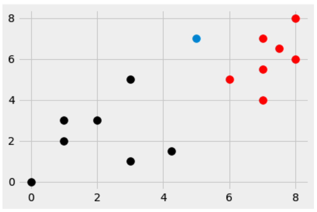
Now, let’s introduce a new dot, the blue one. We’ll place it at [5,7]
import matplotlib.pyplot as plt
from matplotlib import style
style.use('fivethirtyeight')

# Data it bases it's predictions on
dataset = {'k':[[1,2],[3,1],[0,0],[4.25,1.5],[1,3],[2,3],[3,5]], 'r':[[6,5],[7,7],[7,4],[7.5,6.5],[7,5.5],[8,8],[8,6]]}

# Introducing something new
new_features = [5,7]

# One line it
[[plt.scatter(ii[0], ii[1], s=100, color=i) for ii in dataset[i]] for i in dataset];

# Add the new features
plt.scatter(new_features[0], new_features[1], s=100); # Blue

Now for the big question…
Which group does the new blue dot belong in?
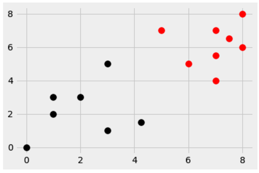
If you say the bottom left, let me know why you say that. As for me, I would classify it to the upper right group, because it’s closer to more of the red dots than black dots.
If you agree with me, congratulations, we’ve basically just done K-Nearest Neighbors.
But wait, what’s the K?
K is whatever you want it to be, but because it often plays the role of a tie breaker, it should always be an odd number. Typically, K defaults at the number 5. But that still doesn’t explain what it is. K is the number of closest dots that vote on what the new dot should be. They try to recruit it to their side.

Let’s Build This Thing With The Cancer Dataset Mentioned Above
The code below will import the data into python for us and we’ll be able to move forward from there.
import pandas as pd

# The column names of the dataset
columns = [
           'id',
           'Clump Thickness',
           'Uniformity of Cell Size',
           'Uniformity of Cell Shape',
           'Marginal Adhesion',
           'Single Epithelial Cell Size',
           'Bare Nuclei',
           'Bland Chromatin',
           'Normal Nucleoli',
           'Mitoses',
           'Class'
           ]

url = 'https://archive.ics.uci.edu/ml/machine-learning-databases/breast-cancer-wisconsin/breast-cancer-wisconsin.data'

df = pd.read_csv(url, names=columns)
df.replace('?', -99999, inplace=True)
df.drop(['id'], axis=1, inplace=True)

# A function with a big long name
def replace_spaces_with_underscore_in_column_names_and_make_lowercasee(df):
  """
  Accepts a dataframe.
  Alters column names- replacing spaces with '_' and column names lowercase.
  Returns a dataframe.
  """
  labels = list(df.columns)
  for i in range(len(df.columns)):
    labels[i] = labels[i].replace(' ', '_')
    labels[i] = labels[i].lower()
  df.columns = labels

  return df

# Invokes the function
df = replace_spaces_with_underscore_in_column_names_and_make_lowercasee(df)

# Shows a dataframe
print(df)
Splitting The Dataframe
Now we need to split dataset into what we’ll call “train/test/split” which will give us X_train, X_test, y_train, y_test.
# What the model uses to study on
features = df[['clump_thickness',
               'uniformity_of_cell_size',
               'uniformity_of_cell_shape',
               'marginal_adhesion',
               'single_epithelial_cell_size',
               'bare_nuclei',
               'bland_chromatin',
               'normal_nucleoli',
               'mitoses']].astype(int).values.tolist()

# What the model tries to guess
target = df['class'].astype(int).values.tolist()

# Another import
from sklearn.model_selection import train_test_split

# Preform the split of the data
X_train, X_test, y_train, y_test = train_test_split(features, target, test_size=0.20, random_state=42)
Notice the last line, the test_size parameter is .2. That means we’re setting aside 20% of the data for testing our results (think whether the blue dot should be red or balck). That’s where the X_test and y_test come into play. Conversly, 80% of the data is to be used for training. Hence the name “train/test/split”. (I know, it’s so original!).
The features are all the columns except the target. The target is what we want to be able to predict.
Standardizing
What does standardizing mean? In short, it’s bringing all the numbers closer. “Standardization makes all variables to contribute equally to the similarity measures.” We’ll only do this to the X_stuff though.
# Another import
from sklearn.preprocessing import StandardScaler

# Standardize the X stuff
scaler = StandardScaler()
X_train = scaler.fit_transform(X_train)
X_test = scaler.transform(X_test)
WAIT! Lets Cheat Real Quick
This code will give us a glimps of what we should expect when we’ve finished building our own class.
Lets run it, and then walk through it real quick.
# Even more imports
from sklearn.metrics import accuracy_score
from sklearn.neighbors import KNeighborsClassifier

model = KNeighborsClassifier(n_neighbors=5)
model.fit(X_train, y_train)
s_pred = model.predict(X_test)
acc_score = accuracy_score(y_test, s_pred)
print(f'The sklearn accuracy: {acc_score}')
output:
The sklearn accuracy: 0.9714285714285714
Okay, so what just happened? First of all, we had some imports to bring in. Then we instantiated our model, telling it to use the nearest 5 points by saying n_neighbors=5.
Then we had to fit it, which basically takes all the training data and crunches it down so we can have it ready for when it’s needed next.
After fitting the model (the learning phase), we’ll need to get what the computer thinks the predictions ought to be - we’ll call it s_pred which will stand for sklearns prediction.
Next we come to generating an accuracy score (followed by printing it, which we see above). How well did SKLEARN do? Comparing the actual predictions to the generated ones, sklearn was 97.14% correct at “assigning the blue dots to the correct category” or in this case, 97.14% correctly identified the 20% we held out. Predicting which people had cancer, and which didn’t.
Building Our Own Model To Try And Do The Same Thing
import numpy as np

class KNN:
    X_train = None
    y_train = None
    def __init__(self, K):
        self.K = K

    def fit(self,X_train,y_train):
        self.X_train = X_train
        self.y_train = y_train

    def euclidean_distance(self, row1, row2):
        return np.linalg.norm(row1-row2)

    def predict(self, pred):

        # Empty list
        predictions = []

        # Go through each row
        for p in pred:

            # Empty list
            distances = []

            # Every row in the training set
            for i, v in enumerate(self.X_train):

                # Get euclidean distance
                distance = self.euclidean_distance(v, p)

                # Append distance to list
                distances.append([distance, i])

            # Sort smallest to biggest
            sorted_distances = sorted(distances)

            # Slice getting K distances
            k_distances = sorted_distances[:self.K]

            # Predicted what it will be
            predict = [self.y_train[i[1]] for i in k_distances]

            # Tally the votes
            result = max(set(predict), key = predict.count)

            # Append result to the predictions list
            predictions.append(result)

        # return the prediction
        return predictions
That’s a lot of code, lets look closer at it.
It’s a class, which starts off by setting X_train and y_train to None. They’ll come into play later.
Every class needs an __init__ method, kinda like the class clown, somebody’s gotta fill the roll. The __init__ basically accepts K from the user.
Then we’ve got the fit method, this is where the chrunching of the X_train and y_train come into play.
It’s followed by the euclidean_distance method, which does some fancy math (linear algebra) to figure out how far away each point is from the other, think how far the blue dot is from every other dot… (Remember the blue dot above?)
Next, and lastly comes the predict method, which was the hardest for me to figure out. But if you’ve followed along with everything I’ve said up to this point, the predict method shouldn’t be that scary.
Lets go backwards explaining this, starting at the bottom.
Starting at the end, it returns predictions in the form of a list, which comes from the different points (think dots above) voting on who should join them. It’s limited to only the closest K (5 in this case) which come from measuring the distance from every point in the training data.
Phew! That’s a lot!
Let’s Test The Class
Because we’ve seen this kind of code above, I won’t explain every line.
model = KNN(K=5)
model.fit(X_train, y_train)
y_pred = model.predict(X_test)
my_acc_score = accuracy_score(y_test, y_pred)

print(f'My Class Accuracy: {my_acc_score}')
First we instantiate our model using the class we just made, then, just like whe we ran it with sklearn’s model, we fit, predict and get an accuracy score.
Conclusion
Let’s run it and see what our score is, we’ll use the same training data and the same testing data as above whe we ran it for the sklearn model.
And we get…
output
My Class Accuracy: 0.9714285714285714
The same exact score as the sklearn model! How amazing is that.
Hopefully you understand K-Nearest Neighbors a bit better now. I know I sure do!
My code can be found here
KNN Documentation
The sklearn’s KNN class can be found here
UCI Breast Cancer Wisconsin (Original) Data Set